Reinforcement Learning (Machine Learning)

Introduction

Reinforcement Learning is a type of unsupervised learning algorithm that focuses on optimizing the path to a desired outcome by maximizing the reward and minimizing the penalty. Or according to Wikipedia:

Reinforcement learning (RL) is an area of machine learning concerned with how intelligent agents ought to take actions in an environment in order to maximize the notion of cumulative reward.

What Defines Reinforcement Learning?

There are a number of factors that define a reinforcement learning model:

The input is the initial state of the model.
The output has a vast number of possibilities.
The model is trained by making a decision and is then rewarded or penalized until a prescribed outcome is reached.
The optimal outcome is derived from the outcome with the highest reward.
The model can continue to learn.
Decisions are dependent, so sequences of dependent decisions are labeled.

There are also a number of practical, real-world applications of reinforcement learning that are worth noting:

Autonomous Machines and robotics
Machine Learning and Data Processing
Generating Custom Instructions
Any environment in which information is collected by making interactions

Q-Learning

Introduction to Q-Learning

Q-Learning is a reinforcement learning technique that uses a reward matrix or Q-matrix to demonstrate states, actions, and rewards. The Q-matrix varies in each different implementation, as it consists of a row for each possible state and a corresponding column for each possible action at the state.

To generate the Q-matrix, Python's NumPy library is used as shown below. You will initialize the matrix with zeroes to begin so that you can update each action with a corresponding reward later. Use the following code to set the state_size and action_size to the desired row and column amounts, respectively.

import numpy as np
Q_Matrix = np.zeros((state_size, action_size))
print(Q_Matrix)

There are two ways to contribute to the Q-matrix. The first method is referred to as exploring: the algorithm chooses a random state and a random action, then calculates the total cost to reach the reward from there. Exploring is important because it allows the algorithm to find and calculate new states.

The second method is referred to as exploiting: where the algorithm references the Q-matrix for all possible actions. The action with the maximum value will then be chosen as the desired action from that given state. Balancing exploring and exploiting is important and can be controlled by what's commonly referred to as the exploration rate or $ϵ$ .

A table update will be performed for each step and will end when an episode is complete. An episode can be thought of as an endpoint being reached, given a random starting point. The whole table will not be complete with just a single episode, but with enough episodes and exploration, the algorithm will find all optimal Q-values. Q-values are the values that are stored, updated and referenced in the Q-matrix.

Calculating the Q-Learning Algorithm

The steps to perform a Q-Learning algorithm are as follows:

The Q-Learning algorithm starts at some state $S_{1}$ , then takes some action $A_{1}$ to receive a reward $R_{1}$ .
The algorithm chooses an action to take by referencing the Q-matrix and choosing the most rewarding action, or the algorithm chooses an action randomly to fill in more of the Q-matrix. This is decided by the exploration rate $ϵ$ .
After the action is performed and the reward is calculated, the Q-matrix is updated with a formula.

The formula for the Q-learning algorithm is as follows:

$Q [s t a t e, a c t i o n] = Q [s t a t e, a c t i o n] + η \cdot (r e w a r d + γ \cdot M a x (Q [n e w S t a t e, :]) - Q [s t a t e, a c t i o n])$

The above equation has some variables that need to be defined:

$η$
- The $η$ variable is the learning rate of the model.
- This variable dictates the extent to which the newly calculated value is accepted.
- In the Q-learning formula above, you are computing the difference between the new and old values, multiplying it by the learning rate, and then adding the difference to your Q-matrix.
  - This essentially moves you in the direction of the latest action.
$γ$
- Gamma ( $γ$ ) is the discount factor.
- It's used to balance current and future rewards.
- You can see this being applied to the calculated future reward, making it have more or less weight on your current state.
- This variable will generally be between 0.8 and 0.99.
Reward
- A reward is a value given to a certain state after performing an action.
- A reward can be added any time in any state and is dependent on the specific problem that is being solved.
$M a x ()$ function
- The $M a x ()$ function acts as a placeholder to allocate the values of future rewards to the current state.
- You can think of this as a recursive function, as this portion will be greed and choose the best path given all possible actions for that next state.

Bellman Equation

TODO: This needs to be explained better. Use this Wikipedia: Bellman Equation

Implementing Q-Learning

Overview of Algorithm to Create Q-Matrix

Choose a random state.
Find the list of possible actions for that state.
Choose an action at random (or use the matrix to find the best one???).
Update the Q matrix with the Bellman equation.

Example Problem

Pretend there's a robot that has to get out of a house from a specific room. Each room is labelled with a number and the outside "room" is labelled with 5. Below is an image of the rooms with their labels and the doors leading to each one.

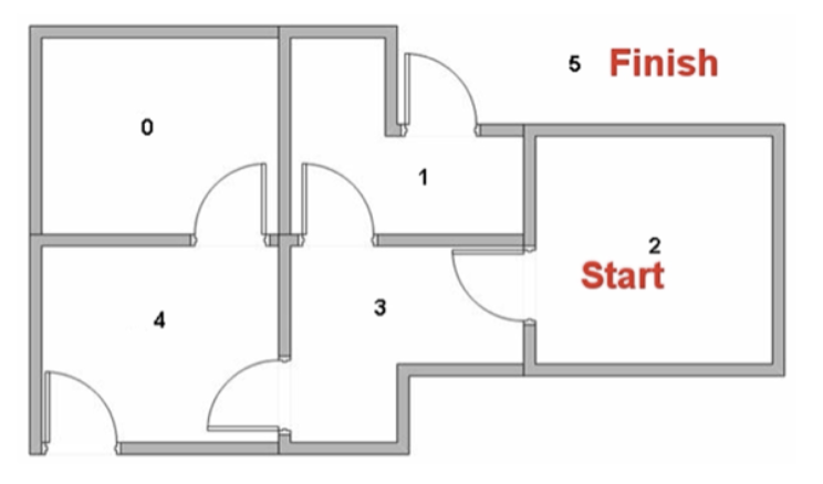
q-learning rooms layout with labels

In this example case we want the robot to be dropped in room 2 and be able to find its way as quickly as possible to room 5 or the outside. Room 5 is accessible through two rooms since the outside is one continuous area surrounding the house.

The connections between each room, which is basically a state is as follows:

0 => 4
1 => 3, 5
2 => 3
3 => 1, 2, 4
4 => 0, 3
5 => 1, 4

Python Implementation of Q-Learning

import numpy aimport numpy as np
# Define the states
ndim = 6
location_to_state = {
    'L0': 0,
    'L1': 1,
    'L2': 2,
    'L3': 3,
    'L4': 4,
    'L5': 5,
}
# Define the actions
actions = [0, 1, 2, 3, 4, 5, 6, 7, 8]
# Define the rewards
rewards = np.array([[0, 0, 0, 0, 1, 0],
                    [0, 0, 0, 1, 0, 100],
                    [0, 0, 0, 1, 0, 0],
                    [0, 1, 1, 0, 1, 0],
                    [1, 0, 0, 1, 0, 100],
                    [0, 1, 0, 0, 1, 100]])

# Maps indices to locations
state_to_location = dict((state, location)
                         for location, state in location_to_state.items())

# Initialize parameters
gamma = 1/2  # Discount factor
alpha = 1.0  # Learning rate


def get_optimal_route(start_location, end_location):
    # Copy the rewards matrix to new Matrix
    rewards_new = np.copy(rewards)

    # Get the ending state corresponding to the ending location as given
    ending_state = location_to_state[end_location]

    # With the above information automatically set the priority of the given ending
    # state to the highest one
    rewards_new[ending_state, ending_state] = 100

    # -----------Q-Learning algorithm-----------

    # Initializing Q-Values
    Q = np.array(np.zeros([ndim, ndim]))
    print(Q)
    np.random.seed(1)
    # Q-Learning process
    for i in range(1000):
        # Pick up a state randomly
        # Python excludes the upper bound
        current_state = np.random.randint(0, ndim)
        # For traversing through the neighbor locations in the maze
        playable_actions = []
        # Iterate through the new rewards matrix and get the actions > 0
        for j in range(ndim):
            if rewards_new[current_state, j] > 0:
                playable_actions.append(j)
        # Pick an action randomly from the list of playable actions
        # leading us to the next state
        next_state = np.random.choice(playable_actions)

        # Compute the temporal difference
        # The action here exactly refers to going to the next state
        TD = rewards_new[current_state, next_state] + gamma * Q[next_state,  
                  np.argmax(Q[next_state, ])] - Q[current_state, next_state]
        # Update the Q-Value using the Bellman equation
        Q[current_state, next_state] += alpha * TD
        #print(f'current: {current_state}, next: {next_state}')
        # print(Q)

 # Initialize the optimal route with the starting location
    route = [start_location]
    # We do not know about the next location yet, so initialize with the value of
    # starting location
    next_location = start_location

    # We don't know about the exact number of iterations
    # needed to reach to the final location hence while loop will be a good choice
    # for iterating

    while(next_location != end_location):
        # Fetch the starting state
        starting_state = location_to_state[start_location]
        # Fetch the highest Q-value pertaining to starting state
        next_state = np.argmax(Q[starting_state, ])
        # We got the index of the next state. But we need the corresponding letter.
        next_location = state_to_location[next_state]
        route.append(next_location)
        # Update the starting location for the next iteration
        start_location = next_location
    print(f'{Q}')
    return route


np.set_printoptions(precision=0)
print(get_optimal_route('L2', 'L5'))

References

Web Links
- Wikipedia.org. 'Reinforcement Learning' Accessed 2023-06-09
- Wikipedia.org. 'Bellman Equation'. Accessed 2023-07-14