NumPy
Short for Numerical Python, is a library that adds support for multi-dimensional arrays, matrices and tensors. NumPy also offers a large collection of high-level mathematical functions, particularly in the fields of linear algebra, statistics and scientific computing.
Import
To import numpy, simply do the regular import statement of the library numpy,
but it's customary to alias it as np so use the as expression to alias it np.
import numpy as npPython List vs NumPy Array
Python lists are mean to be as flexible as possible, thus they can contain just about any data type and that type can vary between list items. This makes Python lists heterogenous and inconsistent. NumPy arrays must allocate space ahead of assigning them, thus its data-types must be consistent and homogenous. The reason NumPy does this is for speed and efficiency. When all the data types are consistent and homogenous the programming can be better optimized for the data. Since numpy gets used to work on large datasets, this is crucial.
Constructing Arrays
NumPy comes with many functions to construct or initialize arrays.
Below is an exmple of arange().
The arange() function works much like the
range() function in python's built-ins.
import numpy as np
a = np.arrange(10)
The array created is just empty uninitialized values.
There might be a need of initial values for all elements of the array.
There's the ones() function which fills it with
the value 1 for each element.
b = np.ones(10)Or there's the np.random submodule of numpy which is full of
functions to construct different random distributions in an array.
Below is an example of the choice function which is a uniform discrete distribution.
c = np.random.choice(np.arange(10, 20, 2))Above you can see how range-like are also valid arguments in many numpy constructors.
And speaking of arange, it's possible to do discrete steps that aren't integers.
In the range(start:stop:step) syntax of python,
in numpy it gets used as well, including with floats.
x = np.arange(0, 10, 0.1)
y = np.sin(x)
It's even possible to create dependent variables like mathematic functions out of
the discrete input created by arange. The variable y above maps the
sine function to the input range stored in x.
Data Shape
Not only must numpy arrays have the same data types and be consistent; they must also have a compatible shape in a lot of operations as well. Consider the below code:
a = np.array([2, 4, 6])
print(a)
print(a.shape)
# output:
# [2 4 6]
# (3,)
This prints out the contents of the array a and
then the shape of it.
Note that the shape is a tuple of size 3 with no other number.
This means it's a one-dimensional array of size 3.
If a array was to substitute this one, it would have to be a
one-dimensional array of size 3 to work.
More of these considerations will come up as you use numpy.
Especially with more advanced methods & functions.
New Arrays from Existing Ones
Indexing & Slicing
Much like how it gets done in Python lists, numpy can slice & index in the same way lists do. The syntax below applies:
a = np.array((0, 1, 2, 3, 4))
b = a[3:0:-1] # b = [3, 2, 1]
c = a[:2] # c = [0, 1, 2]
Again like lists, the syntax is [start:stop:step].
It's also possible to stack vertical and horizontally when
there's more than one dimension.
Stacking
The ndarray methods, vstack and hstack respectively,
will stack arrays in either dimension.
a = np.array([ [1, 1], [2, 2]])
b = np.array([ [3, 3], [4, 4]]))
np.vstack((a, b))
# array([[1, 1],
#       [2, 2],
#       [3, 3],
#       [4, 4]])
np.hstack((a, b))
# array([[1, 1, 3, 3],
#        [2, 2, 4, 4]])
Splitting
You can split an array into smaller arrays using the ndarray hsplit method.
First let's demonstrate by creating a 2x12 array.
>>> x = np.arange(1, 25).reshape(2, 12)
>>> x
array([[ 1,  2,  3,  4,  5,  6,  7,  8,  9, 10, 11, 12],
       [13, 14, 15, 16, 17, 18, 19, 20, 21, 22, 23, 24]])
If you wanted to split this array into 3 equal parts:
np.hsplit(x, 3)[array([ [ 1, 2, 3, 4], [13, 14, 15, 16]]),
array([ [ 5, 6, 7, 8],[17, 18, 19, 20]]),
array([ [ 9, 10, 11, 12],[21, 22, 23, 24]])]But, there's a unique quality going on here, unique to ndarrays, this split is in fact a view...
Views & Copies
Normally sliced lists are copies of the originating list. In numpy arrays, they are views, essentially an object reference. This is because numpy arrays are often used for big data analysis. Having large copies passed around everywhere could become a memory problem. Importantly, these views when assigned to another name will make changes to the original data when the new namespace makes alterations.
>>> a = np.array([ [1, 2, 3, 4], [5, 6, 7, 8], [9, 10, 11, 12]])
>>> b1 = a[0, :]
>>> b1
array([1, 2, 3, 4])
>>> b1[0] == 99
>>> b1
array([99, 2, 3, 4])
>>> a
array([[99,  2,  3,  4],
       [ 5,  6,  7,  8],
       [ 9, 10, 11, 12]])
In the example above,
the array a1 is a 3x4 array counting in row major order.
Variable b1 is a slice or view into the first row of a.
When b1 assigns 99 to b1[0], then a[0][0] reflects that change.
To make a copy,
simply use the copy() method and it will return a deep copy of
the array or slice. This is different from shallow copies,
which describes every view.
The most important thing to remember is that:
When slicing an array, keep in mind whether you need to copy it afterwards or want their changes to affect the original data.
Broadcasting
In numpy milieu, broadcasting refers to array arithmetic between arrays of the same shape and size. This is perhaps best explained through examples.
>>> a = np.array([1, 2, 3])
>>> b = np.array([1, 1, 1])
>>> a + b
np.array([2, 3, 4])
When the shape is the same between ndarrays, basic arithmetic operators run along the ndarrays element-wise. This means the addition above is broadcast along the entire array. A similar broadcast is possible on 0-dimensional arrays or scalar values.
>>> a = np.array([1, 2, 3])
>>> c = 2
>>> a * c
np.array([2, 4, 6])
Because there is no shape to the scalar value 2 above,
it gets broadcast across all the elements of array a.
So when multiplying an ndarray with a scalar value,
the doubling multiplication is broadcasted to every element.
The shape of ndarray operands is crucial when broadcasting operations. The below example shows what happens when incompatible array shapes get added.
>>> a = np.array([1, 2, 3])
>>> a.shape
(3,)
>>> b = np.array([1, 2])
>>> b.shape
(2,)
>>> c = a + b
>>> c
ValueError:
# A traceback
ValueError: operands of shapes (3,) (2,) can't broadcast together
Array a is 1-dimensional of length 3, b is 1-dimensional of length 2.
There is no way to broadcast the 3 elements of a
onto b so they will get added together.
So what the library does is raise a ValueError
alerting of the shape incompatibility.
Matrices
Creating a Matrix
A matrix is any 2-dimensional ndarray* in numpy. There's many ways to create them. Below is an example of composing them using compatibly shaped rows.
>>> a = [0, 1, 2]
>>> b = [3, 4, 5]
>>> c = [6, 7 , 8]
>>> z = [a, b, c]
>>> z
np.array([0, 1, 2],
         [3, 4, 5],
         [6, 7, 8])
It's also possible to create them by transforming a 1D array
into a 2D ndarray by using its reshape method.
>>> a = np.arange(0, 9)
>>> z = a.reshape(3, 3)
>>> z
array([[0, 1, 2],
       [3, 4, 5],
       [6, 7, 8]])
Accessing & Indexing a Matrix
The indexing methods used in nested lists in standard Python lists gets used to access singular elements within a matrix. The first array, usually represented as a column using row major order, accesses the first ndarray. The second array accessor accesses the second array, usually represented as a row.
>>> a = np.arange(0, 9)
>>> z = a.reshape(3, 3) # Same 3x3 matrix as above example
>>> z[2, 2]
8
>>> z[2]
array([6, 7, 8])
The same slicing index from python lists also apply to ndarrays.
The syntax [start:stop:step],
again defines a slice view of the original ndarray.
Just use the square bracket syntax but separate each dimension by a comma.
Remember, it's only a view and a copy needs to get explicitly invoked.
# from the same 'z' array from the above examples
>>> z[0:3, 0:3:2]
array([[0, 2],
       [6, 8]])
The example shows the same array z used before.
The left side of the comma slices first two column arrays.
The right side of the comma slices the 1st & 2nd row arrays.
There's a lot more fine detail about how ndarrays handle matrix operations, indeed any number of extra dimensions. To read more about it, look at NumPy's documentation on ndarrays.
Iterating a Matrix
A matrix gets iterated much the same way any python collection does. A for loop creates an iterator of the outermost ndarray.
# Same z as above
for x in z:
    print(x)
# stdout:
# [1 2 3]
# [4 5 6]
In the same way as with python collections,
it's possible to modify arrays using the same iterators.
Here we see the enumerate iterator get used to
fill every element with its index value multiplied by its row.
>>> for i, x in enumerate(z):
        for j, y in enumerate(x):
            y = j * (1 + i)
>>> z
array([[0, 1, 2],
       [6, 8, 10],
       [18, 21, 24]])
Filtering an NDArray
This applies to any ndarray,
it's just more useful in larger dimensions.
There's the extract class function to np.
>>> a = np.array([ [1, 2, 3],[4, 5, 6]])
>>> b = np.where(a > 4, a)
>>> b
array([5, 6])
The extract function takes any predicate involving an ndarray
then it runs through every element applying that predicate to each element.
If the predicate is true for the element, it gets extracted & returned.
A predicate is any function that evaluates to true or false.
In the case of ndarrays,
this means the predicate must include an ndarray
as if it represents every element.
The where numpy function does essentially the same thing,
but instead returns the index.
>>> b = np.where(a > 4)
>>> b
array(array([1, 1]), array([1, 2]))
Common Numpy Methods
There's a complete index of NumPy documentation, but here are the most common methods used in NumPy.
| Method | Description |
|---|---|
| np.array(n) | Creates n-dimensional arrays |
| np.zeros(n) | Creates an array of length n with entries that are all zeros |
| np.ones(n) | Creates an array of length n with entries that are all ones |
| np.eye(n) | Creates array sized n w/ 1s on diagonal & 0s elsewhere (id-matrix) |
| np.linspace(a,b,n) | Creates an array with n equally spaced entries from a to b |
| np.random.rand(n) | Creates an array with n random float entries |
| np.random.randint(n) | Creates an array with n random int entries |
Numpy File Handling
Though it's certainly possible to manage files using the standard python means, numpy comes with some funcitons to immediately create ndarrays.
First, there's the numpy.loadtxt funciton.
The most important use of this function is to apply a conv
or converter function to transform the input into an array.
def read_ints(in_str):2D Probability & Frequency in NumPy
Underlying Distribution of an Unknown Population
Imagine a bag of marbles with numbers. You pull out a few marbles in this sequence. "5, 5, 6, 4, 5". You might think that all the numbers are under the number 10. That might not be true, but that is essentially determining the underlying statistics and propbabilities of a population based on a sample population.
Tools for Determining the Underlying Distribution
Numpy allows us to generate distributions. Histograms allow us to understand what the data looks like in the underlying population.
NumPy has a function np.random.choice that allows us to
randomly generate a random sample from a given 1-D array.
Its first argument is the array from which to choose,
it could also be a range like np.arange(10).
Then the second argument is the number of samples to choose.
# Data as sampling from an unseen population
# Choose at random from 0 through 9
import numpy as np
import matplotlib.pyplot as plt
# np.random.seed(69)
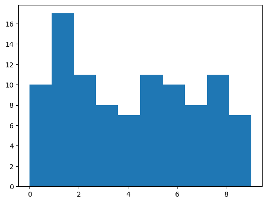
a = np.random.choice(np.arange(0, 10), 100)
print(a)
# Output:
# array([3, 0, 1, 1, 3, 1, 5, 2, 1, 3, 9, 8, 8, 6, 8, 5, 3, 5, 8, 7, 2, 9,
# 3, 9, 2, 1, 4, 3, 3, 0, 9, 2, 9, 4, 6, 4, 9, 0, 1, 7, 7, 9, 1, 1,
# 6, 9, 2, 5, 3, 5, 1, 6, 6, 1, 1, 3, 4, 0, 0, 7, 3, 5, 4, 1, 9, 3,
# 3, 8, 0, 7, 3, 0, 6, 4, 9, 9, 6, 5, 1, 5, 2, 4, 0, 9, 8, 6, 0, 1,
# 5, 8, 9, 9, 4, 7, 8, 7, 9, 8, 9, 4])
plt.hist(a, bins=10)Here you see you get a random set of
numbers from 0 to 9 defined by np.arange(0, 10).
Note that they are each independent trials.
But how do we make sense of the distribution? We may want to know the probability of a number being drawn. Or maybe we want to know the frequency of each number being drawn.
That's where histograms come in. Using matplotlib's hist function, like above you get this histogram plot.
For more information on histograms, using python, see the section on histograms using matplotlib.